Exercise: K-mer and contamination analysis
Exercises:
-
What is a k-mer?
solution
A k-mer is a sequence of length k.
-
Use the following set of commands to extract the list of k-mers in
Bacteria/bacteria_R{1,2}.fastq.gz.mkfifo <named_pipe.fastq> && zcat <reads.fastq.gz> > <named_pipe.fastq> & # Make a named pipe and run in the background kat hist -t 4 -d -o <output.hist> <named_pipe.fastq> # Run KAT reading from the named pipe kat_jellyfish dump <output.hist>-hash.jf27 > <kmer.lst> # Use Jellyfish to print out a human readable list rm <named_pipe.fastq> # named pipes can only be used once, and so are removed after use.The **
** file has the following format. >frequency kmer_sequenceHow many distinct k-mers were found? Use the line count command
wc -lto find out.solution
mkfifo sequences.fastq && zcat bacteria_R{1,2}.fastq.gz > sequences.fastq & kat hist -t 4 -d -o bacteria.hist sequences.fastq kat_jellyfish dump bacteria.hist-hash.jf27 > kmer.lst rm sequences.fastq paste - - < kmer.lst | wc -l 41531545 - How many k-mers have a frequency of 1? Use the following command to find out.
 paste - - < kmer.lst | cut -c2- | awk '$1 == 1 { sum++ } END { print sum+0 }'
 # paste - - : reads two consecutive lines onto the same line.
 # cut -c2- : prints from the second character up to the last character in a line.
 # awk '$1 == 1 { sum++ } END { print sum+0 }' : if column 1 has a frequency of 1, increase the variable "sum". Print the value of "sum" at the end.
solution
35701246
-
How many k-mers have a frequency greater than 5?
solution
paste - - < kmer.lst | cut -c2- | awk '$1 > 5 { sum++ } END { print sum+0 }' 4969071 -
A k-mer histogram was plotted using
kat histin a file*.hist.png. Open the image usingdisplayand estimate the mean k-mer frequency.solution
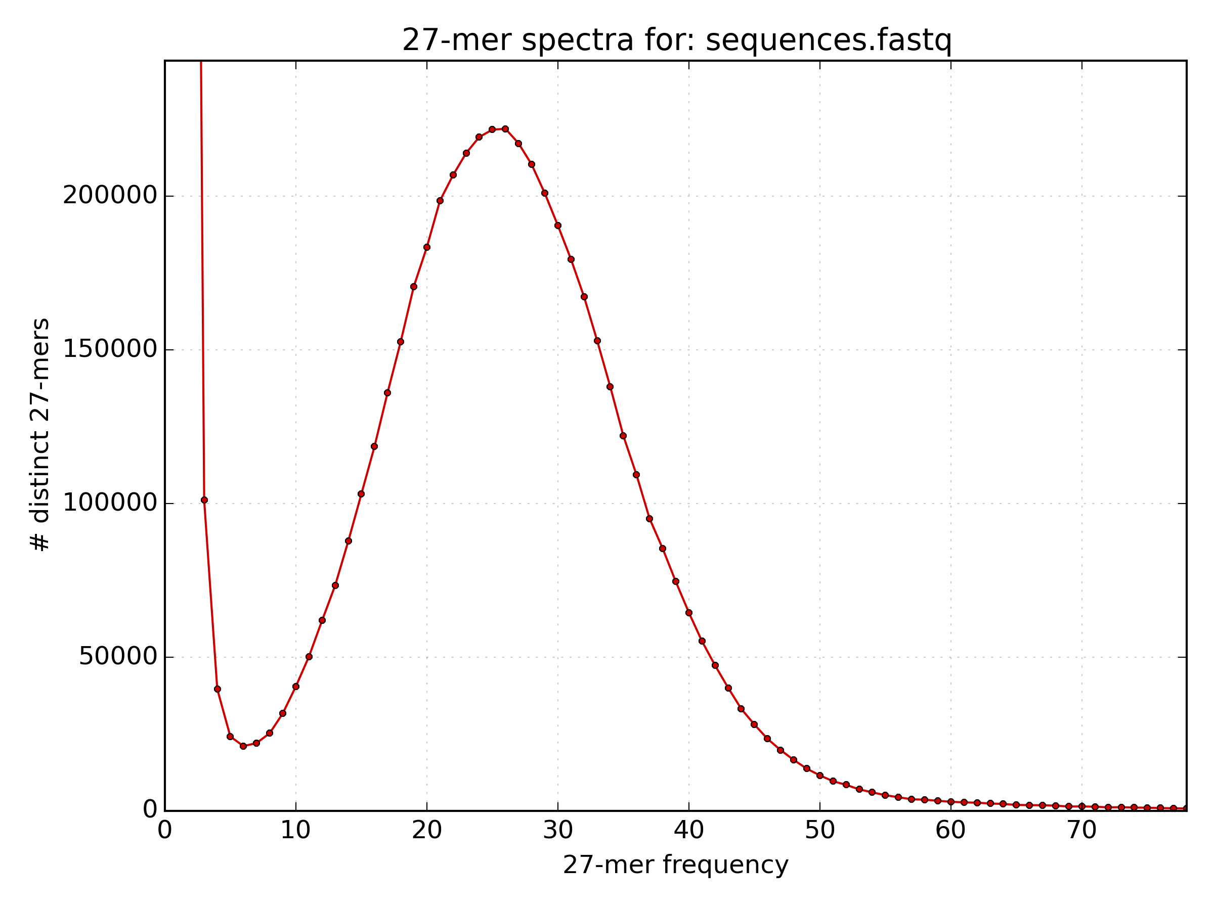 The mean k-mer frequency appears to be around 25.
 - The following command prints the frequency of each k-mer frequency between 5 and 45. What is the mean k-mer frequency?
 paste - - < kmer.lst | cut -c2- | awk '$1 > 5 && $1 < 45 {sum[$1]++ } END { for (freq in sum) {print freq" "sum[freq]} }' | sort -k1,1n
 # paste - - : reads two consecutive lines onto the same line.
 # cut -c2- : prints from the second character up to the last character in a line.
 # awk '$1 > 5 && $1 < 45 {sum[$1]++ } END { for (freq in sum) {print freq" "sum[freq]} }' :
 # 	if column 1 has a frequency greater than 5 and less than 45, increase the value of the array "sum[frequency]" by 1.
 # 	Then for each frequency in sum print the value of sum[frequency] at the end.
 # sort -k1,1n : Perform a numerical sort on the data sorted only by column 1
solution
The mean k-mer frequency is the k-mer frequency (column 1) with the highest count (column 2), which is 26.
- Use
kat gcpto plot the gc content vs k-mer frequency.mkfifo <named_pipe.fastq> && zcat <reads.fastq.gz> > <named_pipe.fastq> & # Make a named pipe and run in the background kat gcp -t 4 -o <output.gcp> <named_pipe.fastq> # Run KAT reading from the named pipe rm <named_pipe.fastq> # named pipes can only be used once, and so are removed after use.Open the plot of GC vs coverage. On what scale is the GC content measured and how is this converted to GC%?
solution
mkfifo sequences.fastq && zcat bacteria_R{1,2}.fastq.gz > sequences.fastq & kat gcp -t 4 -o bacteria.gcp sequences.fastq rm sequences.fastq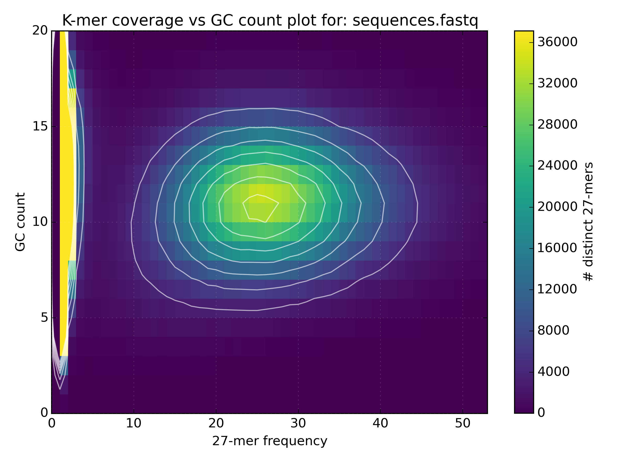 The scale of GC content is the k-mer size, which is in this case 27 (Note: The image
does not go all the way to 27 since the y-axis has been cropped for some reason).
In order to find GC%, one should multiply the GC count by 100% divided by the k-mer size
(e.g. the mean GC count is at 11, and so the mean GC% is 11 * 100 / 27 = 40.74%).
The scale of GC content is the k-mer size, which is in this case 27 (Note: The image
does not go all the way to 27 since the y-axis has been cropped for some reason).
In order to find GC%, one should multiply the GC count by 100% divided by the k-mer size
(e.g. the mean GC count is at 11, and so the mean GC% is 11 * 100 / 27 = 40.74%). - Use
kat compto compareBacteria/bacteria_R{1,2}.fastq.gz.mkfifo <named_pipe_read1.fastq> && zcat <read1.fastq.gz> > <named_pipe_read1.fastq> & # Make a named pipe for read 1 and run in background mkfifo <named_pipe_read2.fastq> && zcat <read2.fastq.gz> > <named_pipe_read2.fastq> & # Make a named pipe for read 2 and run in background kat comp -t 4 -o <output.cmp> --density_plot <named_pipe_read1.fastq> <named_pipe_read2.fastq> # run KAT on the named pipes and print a density plot kat plot spectra-mx -x 50 -y 500000 -i -o <output.cmp>-main.mx.spectra-mx.png <output.cmp>-main.mx # Make a spectra-mx plot rm <named_pipe_read1.fastq> <named_pipe_read2.fastq> # names pipes can only be used once, and so are removed after useWhy is there a difference in the distribution means between the two datasets?
solution
 mkfifo read1.fastq && zcat bacteria_R1.fastq.gz > read1.fastq &
 mkfifo read2.fastq && zcat bacteria_R2.fastq.gz > read2.fastq &
 kat comp -t 4 -o bacteria_R1vR2.cmp --density_plot read1.fastq read2.fastq
 kat plot spectra-mx -x 50 -y 500000 -i -o bacteria_R1vR2.cmp-main.mx.spectra-mx.png bacteria_R1vR2.cmp-main.mx
 rm read1.fastq read2.fastq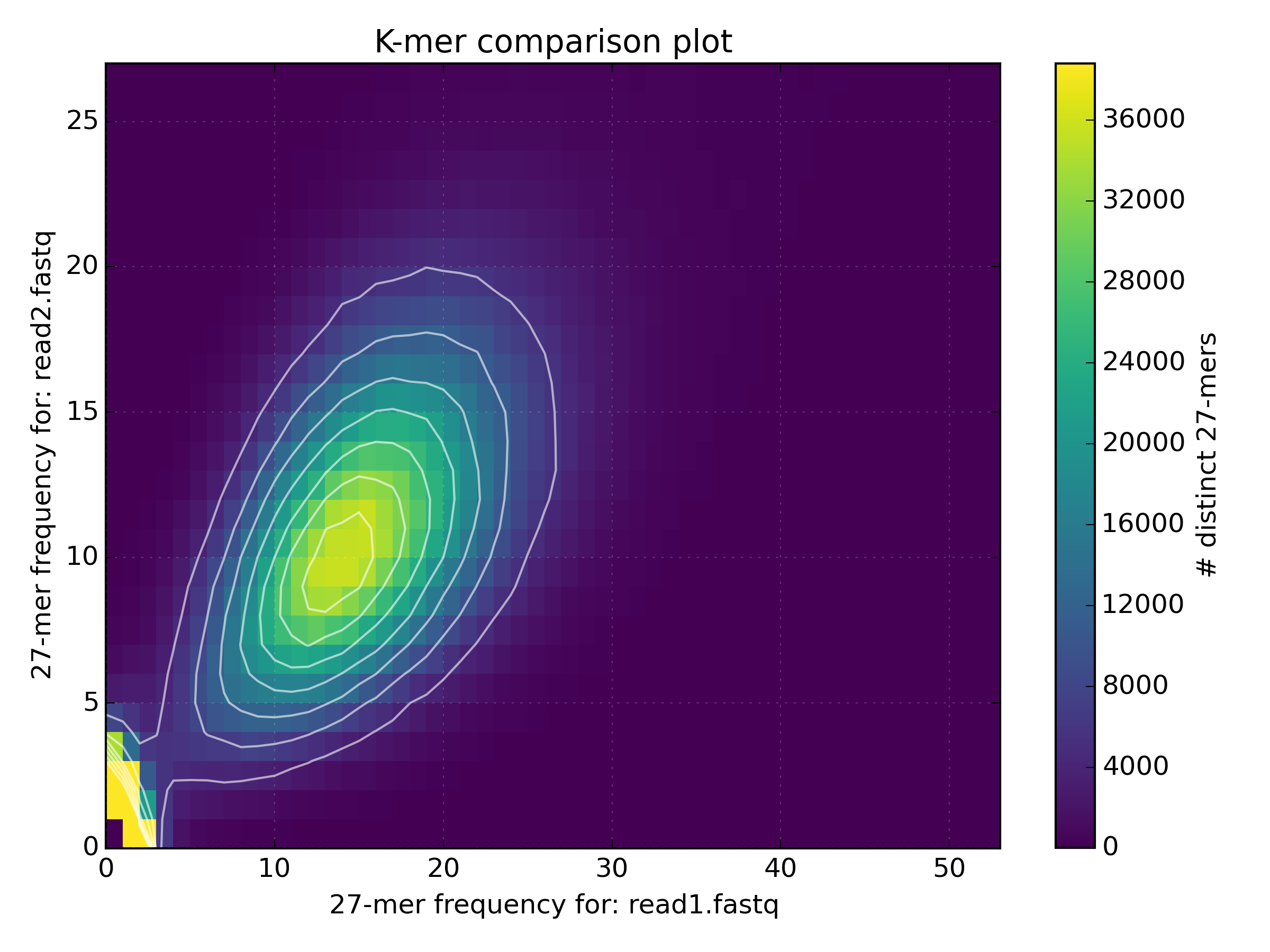
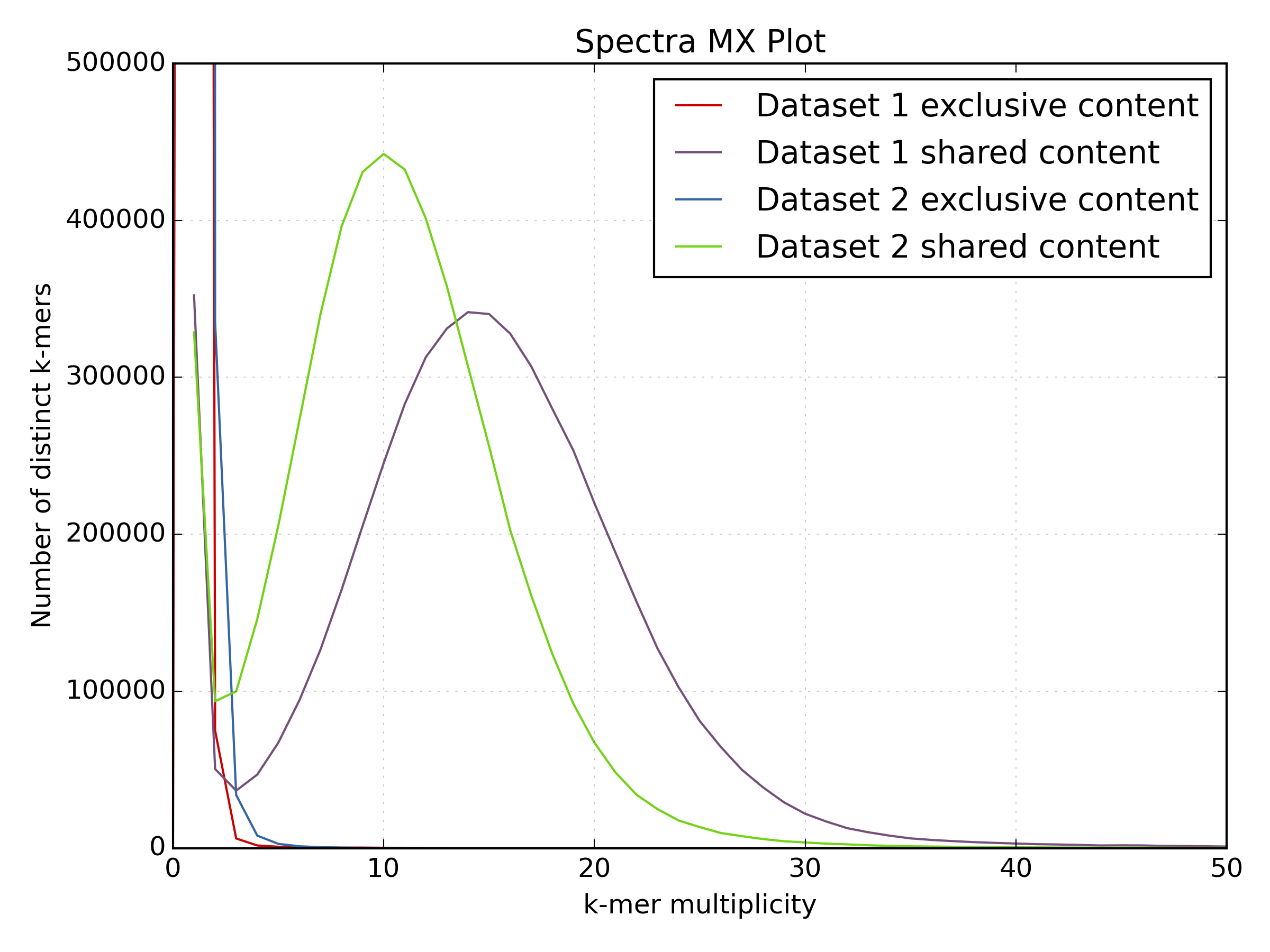
The difference in the distribution means between the two datasets is due to the lower quality of the second read file. The increased number of reads with N’s reduces the k-mer count frequency as k-mers with N are not included in the plot. This increases the number of k-mers with lower k-mer frequency.
- Run Kraken on
Bacteria/bacteria_R{1,2}.fastq.gz. What is the reason for this result? Can one do better?KRAKEN_DB=/sw/courses/assembly/minikraken_20141208 kraken --threads 4 --db $KRAKEN_DB --fastq-input --gzip-compressed --paired <read_{1,2}.fastq.gz> > <kraken.out> kraken-report --db $KRAKEN_DB <kraken.out> > <kraken.rpt> cut -f2,3 <kraken.out> > <krona.in> ktImportTaxonomy <krona.in> -o <krona.html>note:
ktImportTaxonomyis now a broken link. Use this file instead:/sw/apps/bioinfo/Krona/2.7/src/KronaTools-2.7/scripts/ImportTaxonomy.plsolution
 kraken --threads 4 -db $KRAKEN_DB --fastq-input --gzip-compressed --paired bacteria_R{1,2}.fastq.gz > bacteria.kraken.out
 kraken-report -db $KRAKEN_DB bacteria.kraken.out > bacteria.kraken.rpt
 cut -f2,3 bacteria.kraken.out > bacteria.krona.in
 /sw/apps/bioinfo/Krona/2.7/src/KronaTools-2.7/scripts/ImportTaxonomy.pl bacteria.krona.in -o bacteria.krona.html
Here you see that very little is identified, indicating that the organism is not in the database. As a result, the other organisms it has identified are likely to be false positives. One could make this better by using the full database.
-
Run Kraken on
Ecoli/E01_1_135x.fastq.gz. What do you find here and how does the error rate influence this finding?solution
kraken --threads 4 -db $KRAKEN_DB --fastq-input --gzip-compressed E01_1_135x.fastq.gz > Ecoli.kraken.out
kraken-report -db $KRAKEN_DB Ecoli.kraken.out > Ecoli.kraken.rpt
cut -f2,3 Ecoli.kraken.out > Ecoli.krona.in
/sw/apps/bioinfo/Krona/2.7/src/KronaTools-2.7/scripts/ImportTaxonomy.pl Ecoli.krona.in -o Ecoli.krona.html
Here you see quite a lot of the sequences identified as E. coli, however due to the increased error rate per base of the subreads, less reads are accurately classified.