File Types
NOTE: in syntax examples, the dollar sign ($) is not to be printed. The dollar sign is usually an indicator that the text following it should be typed in a terminal window.
1. Connecting to UPPMAX
The first step of this lab is to open a ssh connection to UPPMAX. You will need a ssh program to do this:
On Linux: it is included by default, named Terminal.
On OSX: it is included by default, named Terminal.
On Windows: Google MobaXterm and download it.
Fire up the available ssh program and enter the following (replace username with your uppmax user name). -Y means that X-forwarding is activated on the connection, which means graphical data can be transmitted if a program requests it, i.e. programs can use a graphical user interface (GUI) if they want to.
$ ssh -Y username@milou.uppmax.uu.se
and give your password when prompted. As you type, nothing will show on screen. No stars, no dots. It is supposed to be that way. Just type the password and press enter, it will be fine.
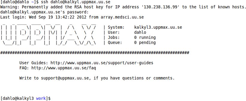
Now your screen should look something like this:
2. Getting a node of your own
()
Usually you would do most of the work in this lab directly on one of the login nodes at uppmax, but we have arranged for you to have one core each to avoid disturbances. This was covered briefly in the lecture notes.
$ salloc -A g2015045 -t 07:00:00 -p core -n 1 --no-shell --reservation=g2015045_20151117 &
check which node you got (replace username with your uppmax user name)
$ squeue -u username
should look something like this
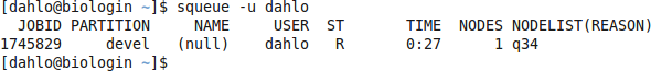
where q34 is the name of the node I got (yours will probably be different). Note the numbers in the Time column. They show for how long the job has been running. When it reaches the time limit you requested (3 hours in this case) the session will shut down, and you will lose all unsaved data. Connect to this node from within uppmax.
$ ssh -Y q34
Note: there is a uppmax specific tool called jobinfo that supplies the same kind of information as squeue that you can use as well ($ jobinfo -u username).
3. Copying files needed for laboratory
To be able to do parts of this lab, you will need some files.
To avoid all the course participants editing the same file all at once, undoing each other’s edits, each participant will get their own copy of the needed files.
The files are located in the folder /proj/g2015045/labs/filetypes
Next, copy the lab files from this folder. -r means recursively, which means all the files including sub-folders of the source folder. Without it, only files directly in the source folder would be copied, NOT sub-folders and files in sub-folders.
NOTE: Remember to tab-complete to avoid typos and too much writing.
Ex.
$ cp -r <source> <destination>

$ cp -r /proj/g2015045/labs/filetypes ~/glob/ngs-intro/
Have a look in ~/glob/ngs-intro/uppmax_tutorial:
$ cd ~/glob/ngs-intro/filetypes
$ tree
This will print a file tree, which gives you a nice overview of the folders where you are standing. As you can see, you have a couple of files and a couple of empty folders. In the 0_ref folder you have a reference genome in fasta format and annotations for the genome in GTF format. In 0_seq you have a fastq file containing the reads we will align.
4. Running a mini pipeline
The best way to see all the different file formats is to run a small pipeline and see which files we encounter along the way. The pipeline is roughly the same steps you’ll do in the resequencing part of the course, so the focus now is not to learn how the programs work. The data is from a sequencing of the adenovirus genome, which is tiny compared to the human genome (36kb vs 3gb).
The starting point of the pipeline is reads fresh from the sequencing machine in fastq format, and a reference genome in fasta format. The goal of the exercise is to look at our aligned reads in a genome viewer together with the annotations of the adenovirus genome.
First, let’s go through the steps of the pipeline:
- Build an index for the reference genome.
- This will speed up the alignment process. Not possible to do without it.
- Align the reads.
- Yepp.
- Convert the SAM file to a BAM file.
- We want to use the space efficiently.
- Sort the BAM file.
- We have to sort it to be able to index it.
- Index the BAM file.
- We have to index it to make it fast to access the data in the file.
- View the aligned data together with the annotations.
Before we do any steps, we have to load the modules for the programs we will be running.
$ module load bioinfo-tools bwa/0.7.8 samtools/1.1 IGV/2.3.17
1. Building an index
- Build an index for the reference genome.
- Align the reads.
- Convert the SAM file to a BAM file.
- Sort the BAM file.
- Index the BAM file.
- View the aligned data together with the annotations.
All aligners will have to index the reference genome you are aligning your data against. This is only done once per reference genome, and then you reuse that index whenever you need it. All aligners have their own kind of index unfortunately, so you will have to build one index for each aligner you want to use. In this lab we will use BWA, so we will build a BWA index.
First, have a look in the 0_ref folder
$ ll 0_ref
You should see 2 files: the fasta file, the gtf file. Have a look at each of them with less, just to see how they look inside.
Syntax: bwa index <name of the fasta file you want to index>

$ bwa index 0_ref/ad2.fa
Since the genome is so small this should only take a second or so. The human genome will probably take a couple of hours.
Look in the 0_ref folder again and see if anything has changed.
$ ll 0_ref
The new files you see are the index files created by BWA. We are now ready to align our reads.
2. Align the reads
- Build an index for the reference genome.
- Align the reads.
- Convert the SAM file to a BAM file.
- Sort the BAM file.
- Index the BAM file.
- View the aligned data together with the annotations.
Now we have a reference genome that has been indexed, and reads that we should align. Do that using BWA, and give the arguments
Syntax: bwa aln <reference genome> <fastq file with reads> > <name of the output file>

$ bwa aln 0_ref/ad2.fa 0_seq/ad2.fq > 1_alignment/ad2.sai
For some reason BWA doesn’t create a SAM file directly. It creates a .sai file which contains only the coordinates for where each read aligns. This format can’t be used by any other program, so we have to convert it to a SAM file. For this, we have to give the program the reference genome we aligned to, the reads we aligned, and the .sai file. It will use the data stored in these files to construct a SAM file.
Syntax: bwa samse <reference genome> <the .sai file> <the fastq reads file> > <the sam file>

$ bwa samse 0_ref/ad2.fa 1_alignment/ad2.sai 0_seq/ad2.fq > 1_alignment/ad2.sam
This will create a SAM file in 1_alignment called ad2.sam. Have a look at it with less.
###3. Convert to BAM
- Build an index for the reference genome.
- Align the reads.
- Convert the SAM file to a BAM file.
- Sort the BAM file.
- Index the BAM file.
- View the aligned data together with the annotations.
The next step is to convert the SAM file to a BAM file. This is more or less just compressing the file, like creating a zip file. To do that we will use samtools, telling it that the input is in SAM format (-S), and that it should output in BAM format (-b).
Syntax: samtools view -S -b <sam file> > <bam file>

$ samtools view -S -b 1_alignment/ad2.sam > 2_bam/ad2.bam
Have a look in the 2_bam folder.
$ ll 2_bam
The created BAM file is an exact copy of the SAM file, but stored in a much more efficient format.
4. Sort and index the BAM file
- Build an index for the reference genome.
- Align the reads.
- Convert the SAM file to a BAM file.
- Sort the BAM file.
- Index the BAM file.
- View the aligned data together with the annotations.
A BAM file is taking up much less space than the SAM file, but we can still improve performance. An indexed BAM file is infinitely faster for programs to work with, but before we can index it, we have to sort it since it’s impossible (no gains performance wise) to index an unsorted file.
To sort the BAMf file use the following command:
Syntax: samtools sort <bam file to sort> <prefix of the outfile>

$ samtools sort 2_bam/ad2.bam 3_sorted/ad2.sorted
This will sort the ad2.bam file and create a new BAM file which is sorted, called ad2.sorted.bam. The .bam file ending will be added automatically, so you should not specify it, unless you want your file named ad2.sorted.bam.bam (you don’t).
Now when we have a sorted BAM file, we can index it. Use the command
Syntax: samtools index <bam file to index>

$ samtools index 3_sorted/ad2.sorted.bam
This will create an index named ad2.sorted.bam.bai . It’s nicer to have the .bam and .bai named to the same “prefix”, so rename the .bai file to not have the .bam in its name.
$ mv 3_sorted/ad2.sorted.bam.bai 3_sorted/ad2.sorted.bai
5. View the data with a genome viewer
- Build an index for the reference genome.
- Align the reads.
- Convert the SAM file to a BAM file.
- Sort the BAM file.
- Index the BAM file.
- View the aligned data together with the annotations.
Now that we have to data aligned and prepared for easy access, we will view it in a genome viewer together with the annotations for the genome. Have a look at the annotations file with less.
$ less -S 0_ref/ad2.gtf
The -S will tell less to not wrap the lines, and instead show one line per line. If the line is longer than the window, you can user the left and right arrow to scroll to the left and right. Many tabular files are extremely more readable when using the -S option. Try viewing the file without it and see the difference.
To view the file, we will use the program IGV (Integrated Genome Viewer). You have already loaded the module for this program at the start of the lab, so start it by typing the following command (now we’ll find out if you used -Y in all your ssh connections!):
$ igv.sh
If you notice that IGV over Xforwarding is excruciatingly slow, you can try to use tha web based ThinLinc client instead. Go to the address https://milou-gui.uppmax.uu.se and login with your normal UPPMAX username and password. This will get you a remote desktop on one of the login nodes, and you can open a terminal and run IGV there instead.
This will start IGV. There are 3 files we have to load in IGV. The first is the reference genome. Press the menu button located at “Genomes - Load Genome from File…“ and find your reference genome in 0_ref/ad2.fa.
The second file you have to load is the reads. Press the menu button “File - Load from File…“ and select your 3_sorted/ad2.sorted.bam.
The last fie you have to load is the annotation data. Press “File - Load from File…“ again and select you annotation file in 0_ref/ad2.gtf.
This will show you the reference genome, how all the reads are aligned to it, and all the annotation data. Try zooming in on an area and have a look at the reads and annotations. The figures you see in the picture are all derived from the data in the files you have given it. The reference genome, a fasta file containing the DNA sequence of the reference genome, is visible if you zoom to the smallest level. All the reads are drawn from the data in the BAM file using the chromosome name, the starting position and the ending position of each read. The annotation in GTF format are all plotted using the data in the GTF file. The chromosome name, the starting position, the ending position, and the additional information in the rest of the fields (strand, name of the annotation, etc).
5. Create a CRAM file
The CRAM format is even more efficient than the BAM format. To create a CRAM file, use samtools. Tell samtools that you want CRAM output (-C) and specify which reference genome it should use to do the CRAM conversion (-T)
Syntax: samtools view -C -T <reference genome> <bam file to convert> > <name of cram file>

$ samtools view -C -T 0_ref/ad2.fa 3_sorted/ad2.sorted.bam > 4_cram/ad2.cram
Compare the sizes of the convered BAM file and the newly created CRAM file:
$ ll -h 3_sorted/ad2.sorted.bam 4_cram/ad2.cram
This will list both the files, and print the file size in a human readable format (-h). The CRAM file is roughly 1/3 of the size of the BAM file. This is probably because all the reads in the simulated data has the same quality value (BBBBBBBBBB). Fewer types of quality values are easier to compress, hence the amazing compression ratio. Real data will have much more diverse quality scores, and the CRAM file would be pethaps 0.7-0.8 time the original BAM file.