File Types

NOTE: in syntax examples, the dollar sign ($) is not to be printed. The dollar sign is usually an indicator that the text following it should be typed in a terminal window.

1. Connecting to UPPMAX

The first step of this lab is to open a ssh connection to UPPMAX. You will need a ssh program to do this:

On Linux: it is included by default, named Terminal.

On OSX: it is included by default, named Terminal.

On Windows: Google MobaXterm and download it.

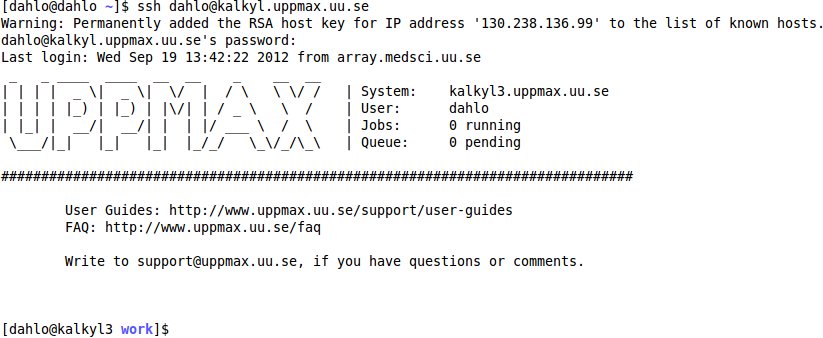
Fire up the available ssh program and enter the following (replace username with your uppmax user name). -Y means that X-forwarding is activated on the connection, which means graphical data can be transmitted if a program requests it, i.e. programs can use a graphical user interface (GUI) if they want to.

$ ssh -Y username@milou.uppmax.uu.se

and give your password when prompted. As you type, nothing will show on screen. No stars, no dots. It is supposed to be that way. Just type the password and press enter, it will be fine.

Now your screen should look something like this:

2. Getting a node of your own

Usually you would do most of the work in this lab directly on one of the login nodes at uppmax, but we have arranged for you to have one core each to avoid disturbances. This was covered briefly in the lecture notes.

$ salloc -A g2018002 -t 02:00:00 -p core -n 1 --no-shell --reservation=g2018002_TUE &

check which node you got (replace username with your uppmax user name)

$ squeue -u username

should look something like this

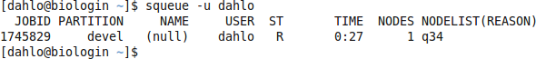
where q34 is the name of the node I got (yours will probably be different). Note the numbers in the Time column. They show for how long the job has been running. When it reaches the time limit you requested (3 hours in this case) the session will shut down, and you will lose all unsaved data. Connect to this node from within uppmax.

$ ssh -Y q34

Note: there is a uppmax specific tool called jobinfo that supplies the same kind of information as squeue that you can use as well ($ jobinfo -u username).

3. Copying files needed for laboratory

To be able to do parts of this lab, you will need some files. To avoid all the course participants editing the same file all at once, undoing each other’s edits, each participant will get their own copy of the needed files. The files are located in the folder /sw/courses/ngsintro/filetypes

Next, copy the lab files from this folder. -r means recursively, which means all the files including sub-folders of the source folder. Without it, only files directly in the source folder would be copied, NOT sub-folders and files in sub-folders.

NOTE: Remember to tab-complete to avoid typos and too much writing.

Ex.

$ cp -r <source> <destination>

$ cp -r /sw/courses/ngsintro/filetypes /proj/g2018002/nobackup/<username>/

Have a look in /proj/g2018002/nobackup/<username>/:

$ cd /proj/g2018002/nobackup/<username>/filetypes
$ tree

This will print a file tree, which gives you a nice overview of the folders where you are standing in. As you can see, you have a couple of files and a couple of empty folders. In the 0_ref folder you have a reference genome in fasta format and annotations for the genome in GTF format. In 0_seq you have a fastq file containing the reads we will align.

4. Running a mini pipeline

The best way to see all the different file formats is to run a small pipeline and see which files we encounter along the way. The pipeline is roughly the same steps you’ll do in the resequencing part of the course, so for now we’ll stick with the dummy pipeline which some of you might have encoutered in the extra material for the UPPMAX exercise. The programs in the dummy pipeline does not actually do any analysis but they work the same way as the real deal, although slightly simplified, to get you familiar with how to work with analysis programs. The data is from a sequencing of the adenovirus genome, which is tiny compared to the human genome (36kb vs 3gb).

The starting point of the pipeline is reads fresh from the sequencing machine in fastq format, and a reference genome in fasta format. The goal of the exercise is to look at our aligned reads in a genome viewer together with the annotations of the adenovirus genome.

First, let’s go through the steps of the pipeline:

1. Build an index for the reference genome.
   • This will speed up the alignment process. Not possible to do the analysis without it.
2. Align the reads.
   • Yepp.
3. Convert the SAM file to a BAM file.
   • We want to use the space efficiently.
4. Sort the BAM file.
   • We have to sort it to be able to index it.
5. Index the BAM file.
   • We have to index it to make it fast to access the data in the file.
6. View the aligned data together with the annotations.

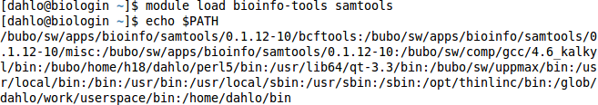
The first thing you usually do is to load the modules for the programs you want to run. During this exercise we’ll only run my dummy scripts that don’t actually do any analysis, so they don’t have a module of their own. What we can do instead is to manually do what module loading usually does: to modify the $PATH variable.

The $PATH variable specifies directories where the computer should look for programs. For instance, when you type

$ nano

how does the computer know which program to start? You gave it the name ‘nano’, but that could refer to any file named nano in the computer, yet it starts the correct one every time. The answer is that it looks in the directories stored in the $PATH variable.

To see which directories that are available by default, type

$ echo $PATH

It should give you something like this, a list of directories, separated by colon signs:

Try loading a module, and then look at the $PATH variable again. You’ll see that there are a few extra directories there now, after the module has been loaded.

$ module load bioinfo-tools samtools/1.3
$ echo $PATH

To pretend that we are loading a module, we will just add a the directory containing my dummy scripts to the $PATH variable, and it will be like we loaded the module for them.

$ export PATH=$PATH:/sw/courses/ngsintro/uppmax_pipeline_exercise/dummy_scripts

This will set the $PATH variable to whatever it is at the moment, and add a directory at the end of it. Note the lack of a dollar sign infront of the variable name directly after “export”. You don’t use dollar signs when assigning values to variables, and you always use dollar signs when getting values from variables.

IMPORTANT: The export command affects only the terminal you type it in. If you have 2 terminals open, only the terminal you typed it in will have a modified path. If you close that terminal and open a new one, it will not have the modified path.

1. Building an index

1. Build an index for the reference genome.
2. Align the reads.
3. Convert the SAM file to a BAM file.
4. Sort the BAM file.
5. Index the BAM file.
6. View the aligned data together with the annotations.

All aligners will have to index the reference genome you are aligning your data against. This is only done once per reference genome, and then you reuse that index whenever you need it. All aligners have their own kind of index unfortunately, so you will have to build one index for each aligner you want to use. In this lab we will use the dummy aligher called align_reads, and we will build a index using it’s indexing progam, called reference_indexer.

First, have a look in the 0_ref folder

$ ll 0_ref

You should see 2 files: the fasta file, the gtf file. Have a look at each of them with less, just to see how they look inside. To do the actual indexing of the genome:

Syntax: reference_indexer -r <name of the fasta file you want to index>

Answer below in white text:

Since the genome is so small this should only take a second or so. The human genome will probably take a couple of hours.

Look in the 0_ref folder again and see if anything has changed.

$ ll 0_ref

The new file you see is the index file created by reference_indexer. This index is in the same format as you would get from the real program samtools. Try viewing the index file with less and see how it looks. The samtools type of index contains one row per fasta record in the reference file. In this case there is only one record for the adenovirus genome, and it’s called ad2 in the fasta file. The human reference genome typically have one record per chromosome, so a index of the human genome would then have 24 rows.

The numbers after the record name specifies how many bases the record has, how far into the file (in bytes) the record starts, the number of bases on each line in the record, and how many bytes each line takes up in the file. Using this information the program can quickly jump to the start location of each record, without having to read the file from the first row every time.

Other aligners might use more complex indexing of the file to speed up the alignment process even further, e.g. creating an index over where it can find all possible “words” that you can form with 5 or so bases, making it easier to find possible matching sites for reads. If the read starts with ATGTT you can quickly look in the index and see all places in the geonome that contains this word and start looking if the rest of the read matches the area around the word.

This greatly decreases the number of places you have to look when looking for a match. These types of indexes usually take a long time to create (5+ hours maybe), but since you only have to do it once per reference genome it’s easily worth it, seeing how the alignment process probably would take 100s of hours without the index, instead of 6-12 hours.

We are now ready to align our reads.

2. Align the reads

1. Build an index for the reference genome.
2. Align the reads.
3. Convert the SAM file to a BAM file.
4. Sort the BAM file.
5. Index the BAM file.
6. View the aligned data together with the annotations.

Now we have a reference genome that has been indexed, and reads that we should align. Do that using align_reads, naming the output file ad2.sam, placed in the 1_alignment folder.

Syntax: align_reads -r <reference genome> -i <fastq file with reads> -o <name of the output file>

Answer below in white text:

This will create a SAM file in 1_alignment called ad2.sam. Have a look at it with less. If you think the file looks messy, add a -S after less to make it stop wrapping long lines, less -S 1_alignment/ad2.sam and scroll sideways using the arrow keys. As you can see there is one row per aligned read in this file. Each row contains information about the read, like the name of the read, where in the reference genome it aligned, and also a copy of the reads sequence and quality score, among other things.

3. Convert to BAM

1. Build an index for the reference genome.
2. Align the reads.
3. Convert the SAM file to a BAM file.
4. Sort the BAM file.
5. Index the BAM file.
6. View the aligned data together with the annotations.

The next step is to convert the SAM file to a BAM file. This is more or less just compressing the file, like creating a zip file. To do that we will use the dummy program sambam_tools, telling it we want to convert a file to BAM (-f bam), which file we want to convert (-i), where it should save the resulting BAM file (-o). Save the BAM file in the 2_bam folder and name it ad2.bam.

Syntax: sambam_tool -f bam -i <sam file> -o <bam>

Answer below in white text:

Have a look in the 2_bam folder.

$ ll 2_bam

The created BAM file is an exact copy of the SAM file, but stored in a much more efficient format. Aligners usually have an option to output BAM format directly, saving you the trouble to convert it yourself, but not all tools can do this (they really should though).

Have a look at the difference in file size, though in this example it’s quite an extreme difference (2.9 MB vs 0.3 MB). The quality score of all reads is the same (BBBBBBBBB..), and files with less differences are easier to compress. Usually the BAM file is about 25% of the size of the SAM file.

Since the BAM format is a binary format we can’t look at it with less. We would have to use a tool, like samtools which you will probably see later in the week, to first convert the file back to a SAM file before we can read it. In that case we can just look at the SAM file before converting it since they will be the same.

4. Sort and index the BAM file

1. Build an index for the reference genome.
2. Align the reads.
3. Convert the SAM file to a BAM file.
4. Sort the BAM file.
5. Index the BAM file.
6. View the aligned data together with the annotations.

A BAM file is taking up much less space than the SAM file, but we can still improve performance. An indexed BAM file is infinitely faster for programs to work with, but before we can index it, we have to sort it since it’s not possible to index an unsorted file in any meaningful way.

To sort the BAM file we’ll use the sambam_tool again, but specifying a different function, -f sort instead. Tell it to store the sorted BAM file in the 3_sorted folder and name the file ad2.sorted.bam

Syntax: sambam_tool -f sort -i <unsorted bam file> -o <sorted bam file>

Answer below in white text:

This will sort the ad2.bam file and create a new BAM file which is sorted, called ad2.sorted.bam.

Now when we have a sorted BAM file, we can index it. Use the command

Syntax: sambam_tool -f index -i <sorted bam file>

Answer below in white text:

This will create an index named ad2.sorted.bam.bai in the same folder as the ad2.sorted.bam file is located. It’s nicer to have the .bam and .bai named to the same “prefix”, so rename the .bai file to not have the .bam in its name.

$ mv 3_sorted/ad2.sorted.bam.bai 3_sorted/ad2.sorted.bai

5. View the data with a genome viewer

1. Build an index for the reference genome.
2. Align the reads.
3. Convert the SAM file to a BAM file.
4. Sort the BAM file.
5. Index the BAM file.
6. View the aligned data together with the annotations.

Now that we have to data aligned and prepared for easy access, we will view it in a genome viewer together with the annotations for the genome. Have a look at the annotations file with less.

$ less -S 0_ref/ad2.gtf

The -S will tell less to not wrap the lines, and instead show one line per line. If the line is longer than the window, you can user the left and right arrow to scroll to the left and right. Many tabular files are much more readable when using the -S option. Try viewing the file without it and see the difference.

To view the file, we will use the program IGV (Integrated Genome Viewer). Before we can do this, we have to load the module for IGV.

NOTE: If you are using a Mac you might have to install the program XQuartz, if you have not already installed that program. By using -Y in your ssh command you enable graphical transfer over ssh, but you will also have to have a program able to receive the graphics in order to display it. This used to be included in OSX, but it was removed for some unclear reason..

$ module load bioinfo-tools IGV/2.3.17

Start it by typing the following command (now we’ll find out if you used -Y in all your ssh connections!):

$ igv.sh

If you notice that IGV over Xforwarding is excruciatingly slow, you can try to use tha web based ThinLinc client instead. Go to the address https://milou-gui.uppmax.uu.se and login with your normal UPPMAX username and password. This will get you a remote desktop on one of the login nodes, and you can open a terminal and run IGV there instead.

Once IGV is started, either using Xforwarding or the remote desktop in your web browser, we are ready to go. There are 3 files we have to load in IGV. The first is the reference genome. Press the menu button located at “Genomes - Load Genome from File…“ and find your reference genome in 0_ref/ad2.fa.

The second file you have to load is the reads. Press the menu button “File - Load from File…“ and select your 3_sorted/ad2.sorted.bam.

The last fie you have to load is the annotation data. Press “File - Load from File…“ again and select you annotation file in 0_ref/ad2.gtf.

This will show you the reference genome, how all the reads are aligned to it, and all the annotation data. Try zooming in on an area and have a look at the reads and annotations. The figures you see in the picture are all derived from the data in the files you have given it.

At the top of the window you have the overview of the current chromosome you are looking at, which tells you the scale you are zoomed at for the moment. When you zoom in you will see a red rectangle apper which shows you which portion of the chromosome you are looking at.

Just below the scale you’ll see the coverage graph, which tells you how many reads cover each position along the reference genome. The colored bands you see here and there are SNPs, i.e. positions where the reads of your sample does not match the reference genome.

All the reads, the larger area in the middle of the window, are drawn from the data in the BAM file using the chromosome name, the starting position and the ending position of each read. When you zoom in more you will be able to see individual reads and how they are aligned.

The annotation in GTF format are all plotted using the data in the GTF file, visible just under all the reads, are shown as blue rectangles.

The reference genome, a fasta file containing the DNA sequence of the reference genome, is visible at the bottom of the window if you zoom to the smallest level so you can see the bases of the genome.

5. Create a CRAM file

The CRAM format is even more efficient than the BAM format. To create a CRAM file we’ll have to use samtools, so we will load the module for it.

$ module load bioinfo-tools samtools/1.3

Tell samtools that you want CRAM output (-C) and specify which reference genome it should use to do the CRAM conversion (-T)

Syntax: samtools view -C -T <reference genome> -o <name of cram file> <bam file to convert>

Answer below in white text:

Compare the sizes of the convered BAM file and the newly created CRAM file:

$ ll -h 3_sorted/ad2.sorted.bam 4_cram/ad2.cram

This will list both the files, and print the file size in a human readable format (-h). The CRAM file is roughly 1/3 of the size of the BAM file. This is probably because all the reads in the simulated data has the same quality value (BBBBBBBBBB). Fewer types of quality values are easier to compress, hence this amazing compression ratio. Real data will have much more diverse quality scores, and the CRAM file would be pethaps 0.7-0.8 of the original BAM file.

If you have been fast to finish this lab and you still have time left (or just can’t get enough of linux stuff), please have a look at the loops lab where you can learn the basics in bash programming using variables, loops and controll statements.