Isoform detection using RNA seq de novo Assembly
There are many programs to do RNA de novo assembly We are going to use one of the open source RNA de novo assemblers called Trinity in this practical. Independent assessment of de novo assembly programs showed that Trinity was one of the best assemblers to use. It is also one of the programs that is being updated and does also have downstream analysis tools.
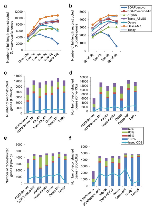
Figure taken from `Optimizing de novo transcriptome assembly from short-read RNA-Seq data: a comparative study.
A de novo assembler takes your reads and turns them into contigs. For more details on how Trinity works, read the corresponding paper.
Preparation
Make a new subdirectory and go there for this exercise.
#Create a new folder where you will do this exercise
mkdir deNovoAssembly
# go into that directory
cd deNovoAssembly
Files used during the exercise
Running an assembly using Trinity for ~20 million of reads takes at least a day and more than 50 GB of RAM. In order to reduce the time for Trinity to run during this course, we will focus on reads that can be mapped to a small region on a human chromosome.
The RNA-seq data comes from 1 experiment with mate pair libraries for sample 1 from the A431 cell line. A description of the dataset can be found here.
To access the data there are two options.
If you are working on uppmax
All the data you need for this lab is available in the folder:
/proj/b2013006/webexport/downloads/courses/RNAseqWorkshop/isoform/deNovo/data/
Copy the data to your folder
cp /proj/b2013006/webexport/downloads/courses/RNAseqWorkshop/isoform/deNovo/data/* .
If you are working from somewhere else
You can download all data using a webinterface from here and put it in your working folder.
You should now have two fastq files in your working folder.
Programs used during the exercise
If you are on uppmax
When doing this course on UPPMAX all programs will be available to load as pre-installed modules. In order to be able to use these programs you need to load the modules before using them.
Load all programs that you will need for trinity to work on uppmax this exercise.
# load modules to make trinity work
module load bioinfo-tools
module load bowtie
module load samtools
module load trinity/2.3.2
If you have not loaded the the STAR module yet to that as well.
# load modules to make RNAseq aligner STAR work
module load star/2.5.1b
If you are somewhere else
If you are doing this exercise on somewhere else follow each program information on how to install it.
Assemble the reads into contigs using trinity
Since Trinity is often being updated you should make sure you are using the latest version. That means that the requirements and the command line to to run Trinity changes occasionally. You can find the basic usage info for Trinity here.
A typical command line to type run trinity looks like this.
Adapt the Trinity command line so it fits with your data and run it.
Good things to know about the data used in this lab :
- You are using fastq files.
- You are using paired end data.
- The RNA-seq data that we use in this exercise is not strand specific.
In general to fully use the potential of a program it is worthwhile to read the manual and use the correct flags. As an example, Trinity handles strand specific RNA-seq data, which reduces the complexity of the algorithm and produces better results.
The minimal line to run that version of trinity is:
Trinity --seqType fq --max_memory 100G --left reads_1.fq --right reads_2.fq --CPU 6
Remember to change the CPU count and memory to it fits with your allocated memory. To get all the available parameters that you can set type:
Trinity --help
Mapping the new assemblies on to a reference genome
Now that the reads have been assembled into contigs you can map them back onto the human genome sequence to see how they were assembled. Note that in non-model organism this is not possible. If you would like to asses the assembly of transcripts without a reference genome, Trinity has a downstream analysis pipeline that is worth following: Trinotate. This is not something we will do in this course but if you have time over feel free to try it out.
Start with mapping the trinity assembled transcripts to the human genome using STAR with the version for long reads (STARlong). Convert them to bam format, sort and index them using samtools:
mkdir STARtrinityMapping

STARlong  --genomeDir /proj/b2013006/webexport/downloads/courses/RNAseqWorkshop/reference/hg19_Gencode14.overhang75  --readFilesIn trinity_out_dir/Trinity.fasta --runThreadN 2 --outSAMstrandField intronMotif --outFileNamePrefix STARtrinityMapping/
samtools sort -o trinityTranscripts.bam STARtrinityMapping/Aligned.out.sam
samtools index trinityTranscripts.bam
When ready there should be a BAM file that is sorted and indexed. It can now be viewed in the IGV genome browser.
In total there were 12 samples and you have now assembled one of those samples. If you want to view all the 12 different samples you can download the assembled and mapped samples. We have also merged the reads from all the 12 samples and used all the reads to create assembled transcripts. On uppmax you can copy the BAM files folder to your folder
cp -r /proj/b2013006/webexport/downloads/courses/RNAseqWorkshop/isoform/otherData/deNovo/BAMfiles/ .
They can also be downloaded from here.
Download a few of them and compare the experiments to see if you can identify different isoforms. How does the de novo assembled transcripts compare to the reference based isoform detection program?
Now that you have all the bam files in with individual names, try to view them in IGV. For how to view files in IGV, see this tutorial.
First have a look on the two bamfiles that contains the assemblies of all
reads from all twelve timepoints with the trinity assemblers. They have the
names RAB11FIP5_trinity.Trinity._hg_19_STAR.bam.
#If you view your files on your laptop start IGV like this

java -Xmx1500M -jar igv.jar

# If you view your files on UPPMAX do according to UPPMAX


#Load tracks in the IGV browser

File->Load From File...
**trinityTranscripts.sorted.bam**

# Load peptide sequences

File->Load From File...
	choose **human_A431_global-TDA-FDR1pc_green-known_red-novel.bed**

# Load your mapped reads from before

File->Load From File...
	choose **sample12_RAB11FIP5.bam**

# Load your own GTF file

File->Load From File...
	choose **transcripts.gtf** or what you have named it.
OPTIONAL There is also a possibility to view tracks that are publicly available. This is easy to do in IGV and adds some information in the region that we are looking into.
# Load different gene annotations files

File->Load From Server...
	choose Available Datasets ->Annotations -> Genes ->UCSC Genes


# Load multiple alignments to other vertebrates

File->Load From Server...
	choose Available Datasets ->Annotations -> Comparative Genomics ->Phastcons (Vertebrate 46 way)
# Load any of the other annotations that you think is interesting
File->Load From Server...
	choose Available Datasets ->..  -> ..  ->Up to you
Now have a look at the de novo assembled transcripts. Do they seem reasonable? Which regions on the de novo assembled transcripts do not correspond to your own .gtf file? Which is the correct one?
Now take a closer look at the region chr2:73,308,166-73,308,278. This corresponds to a region where the “RefSeq genes” track shows an intron but the de novo assembly, the cufflinks gtf file and the peptide file suggest that the region is being transcribed and translated into peptides. When examining the de novo assembled contigs it seems that none of the transcripts goes through the region. Is this real or could there be a shortcoming of the assembler or the sequencing platform? Unfortunately we do not have the answers to these questions but all the different methods add in to give more understanding in the complexity of isoform analysis and genome annotation.